Text classification with tidy data principles

Jane Austen vs. H. G. Wells

Let’s build a supervised machine learning model that learns the difference between text from Pride and Prejudice and text from The War of the Worlds. We can access the full texts of these works from Project Gutenberg via the gutenbergr package.

library(tidyverse)
library(gutenbergr)

titles <- c(
  "The War of the Worlds",
  "Pride and Prejudice"
)
books <- gutenberg_works(title %in% titles) %>%
  gutenberg_download(meta_fields = "title") %>%
  mutate(document = row_number())

books

## # A tibble: 19,504 x 4
##    gutenberg_id text                                 title         document
##           <int> <chr>                                <chr>            <int>
##  1           36 The War of the Worlds                The War of t…        1
##  2           36 ""                                   The War of t…        2
##  3           36 by H. G. Wells [1898]                The War of t…        3
##  4           36 ""                                   The War of t…        4
##  5           36 ""                                   The War of t…        5
##  6           36 "     But who shall dwell in these … The War of t…        6
##  7           36 "     inhabited? .  .  .  Are we or… The War of t…        7
##  8           36 "     World? .  .  .  And how are a… The War of t…        8
##  9           36 "          KEPLER (quoted in The An… The War of t…        9
## 10           36 ""                                   The War of t…       10
## # ... with 19,494 more rows

We have the text data now, and let’s frame the kind of prediction problem we are going to work on. Imagine that we take each book and cut it up into lines, like strips of paper (✨ confetti ✨) with an individual line on each paper. Let’s train a model that can take an individual line and give us a probability that this book comes from Pride and Prejudice vs. from The War of the Worlds. As a first step, let’s transform our text data into a tidy format.

library(tidytext)

tidy_books <- books %>%
  unnest_tokens(word, text) %>%
  group_by(word) %>%
  filter(n() > 10) %>%
  ungroup()

tidy_books

## # A tibble: 159,707 x 4
##    gutenberg_id title                 document word 
##           <int> <chr>                    <int> <chr>
##  1           36 The War of the Worlds        1 the  
##  2           36 The War of the Worlds        1 war  
##  3           36 The War of the Worlds        1 of   
##  4           36 The War of the Worlds        1 the  
##  5           36 The War of the Worlds        3 by   
##  6           36 The War of the Worlds        6 but  
##  7           36 The War of the Worlds        6 who  
##  8           36 The War of the Worlds        6 shall
##  9           36 The War of the Worlds        6 in   
## 10           36 The War of the Worlds        6 these
## # ... with 159,697 more rows

We’ve also removed the rarest words in that step, keeping only words in our dataset that occur more than 10 times total over both books.

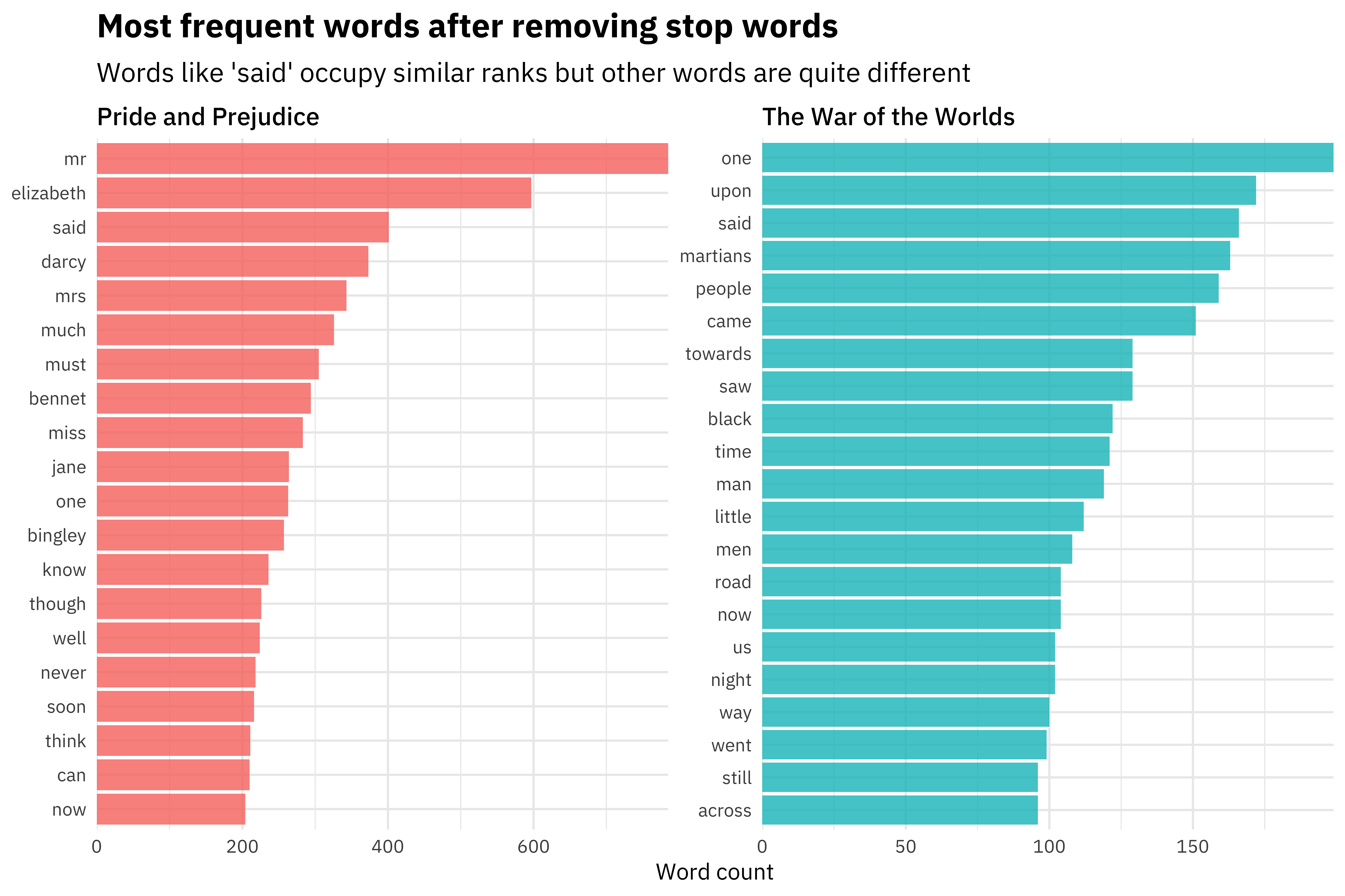
The tidy data structure is a great fit for performing exploratory data analysis, making lots of plots, and deeply understanding what is in the dataset we would like to use for modeling. In interest of space, let’s just show one example plot we could use for EDA, looking at the most frequent words in each book after removing stop words.

tidy_books %>%
  count(title, word, sort = TRUE) %>%
  anti_join(get_stopwords()) %>%
  group_by(title) %>%
  top_n(20) %>%
  ungroup() %>%
  ggplot(aes(reorder_within(word, n, title), n,
    fill = title
  )) +
  geom_col(alpha = 0.8, show.legend = FALSE) +
  scale_x_reordered() +
  coord_flip() +
  facet_wrap(~title, scales = "free") +
  scale_y_continuous(expand = c(0, 0)) +
  labs(
    x = NULL, y = "Word count",
    title = "Most frequent words after removing stop words",
    subtitle = "Words like 'said' occupy similar ranks but other words are quite different"
  )

We could perform other kinds of EDA like looking at tf-idf by book but we’ll stop here for now and move on to building a classification model.

Building a machine learning model

Let’s get this data ready for modeling. We want to split our data into training and testing sets, to use for building the model and evaluating the model. Here I use the rsample package to split the data; it works great with a tidy data workflow. Let’s go back to the books dataset (not the tidy_books dataset) because the lines of text are our individual observations.

library(rsample)

books_split <- books %>%
  select(document) %>%
  initial_split()
train_data <- training(books_split)
test_data <- testing(books_split)

You can also use functions from the rsample package to generate resampled datasets, but the specific modeling approach we’re going to use will do that for us so we only need a simple train/test split.

Now we want to transform our training data from a tidy data structure to a sparse matrix to use for our machine learning algorithm.

sparse_words <- tidy_books %>%
  count(document, word) %>%
  inner_join(train_data) %>%
  cast_sparse(document, word, n)

class(sparse_words)

## [1] "dgCMatrix"
## attr(,"package")
## [1] "Matrix"

dim(sparse_words)

## [1] 12028  1652

We have 12,028 training observations and 1652 features at this point; text feature space handled in this way is very high dimensional, so we need to take that into account when considering our modeling approach.

One reason this overall approach is flexible and wonderful is that you could at this point cbind() other columns, such as non-text numeric data, onto this sparse matrix. Then you can use this combination of text and non-text data as your predictors in the machine learning algorithm, and the regularized regression algorithm we are going to use will find which are important for your problem space. I’ve experienced great results with my real world prediction problems using this approach.

We also need to build a dataframe with a response variable to associate each of the rownames() of the sparse matrix with a title, to use as the quantity we will predict in the model.

word_rownames <- as.integer(rownames(sparse_words))

books_joined <- data_frame(document = word_rownames) %>%
  left_join(books %>%
    select(document, title))

Now it’s time to train our classification model! Let’s use the glmnet package to fit a logistic regression model with LASSO regularization. It’s a great fit for text classification because the variable selection that LASSO regularization performs can tell you which words are important for your prediction problem. The glmnet package also supports parallel processing with very little hassle, so we can train on multiple cores with cross-validation on the training set using cv.glmnet().

library(glmnet)
library(doMC)
registerDoMC(cores = 8)

is_jane <- books_joined$title == "Pride and Prejudice"
model <- cv.glmnet(sparse_words, is_jane,
  family = "binomial",
  parallel = TRUE, keep = TRUE
)

We did it! 🎉 If you are used to looking at the default plot methods for glmnet’s output, here is what we’re dealing with.

plot(model)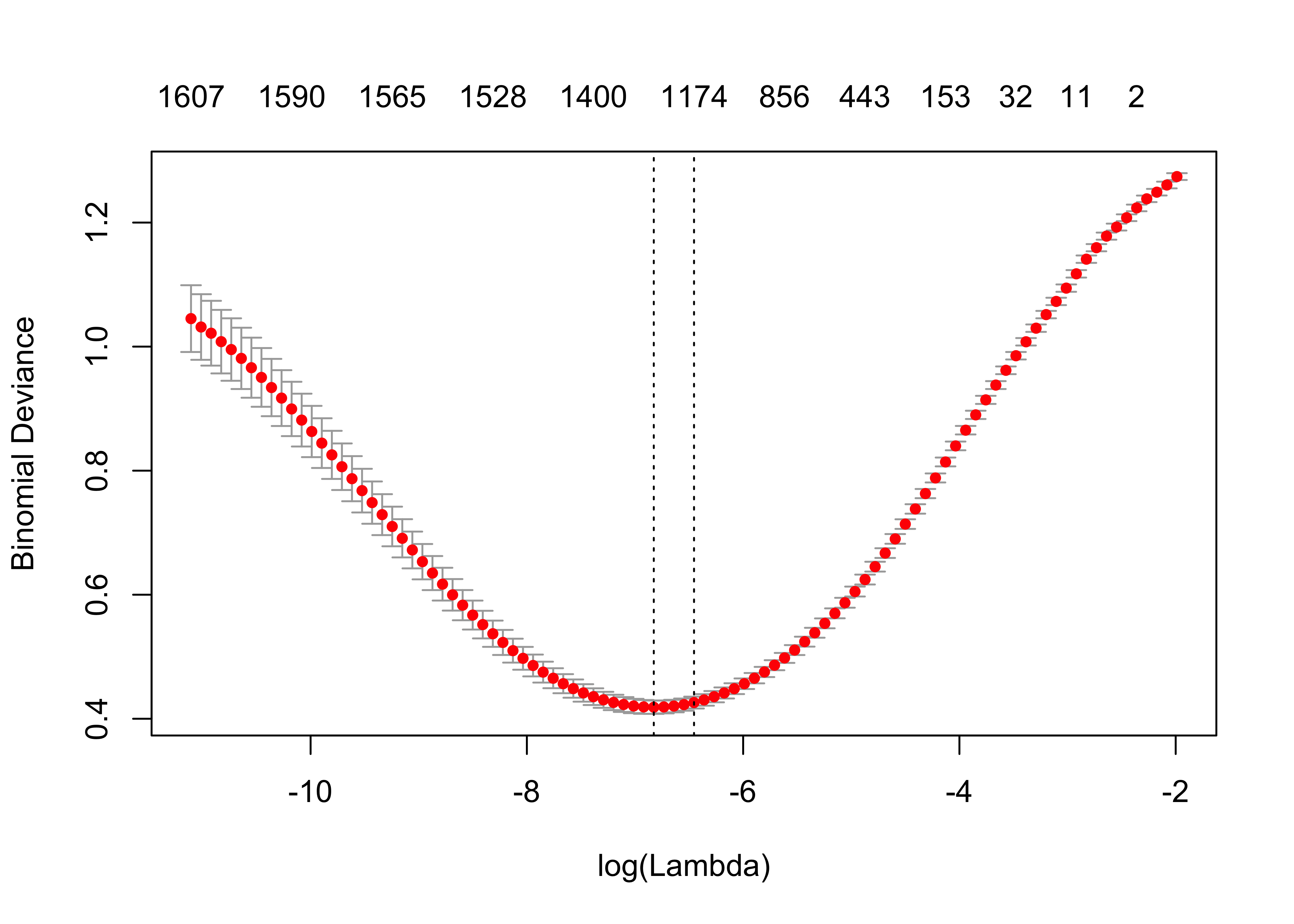

plot(model$glmnet.fit)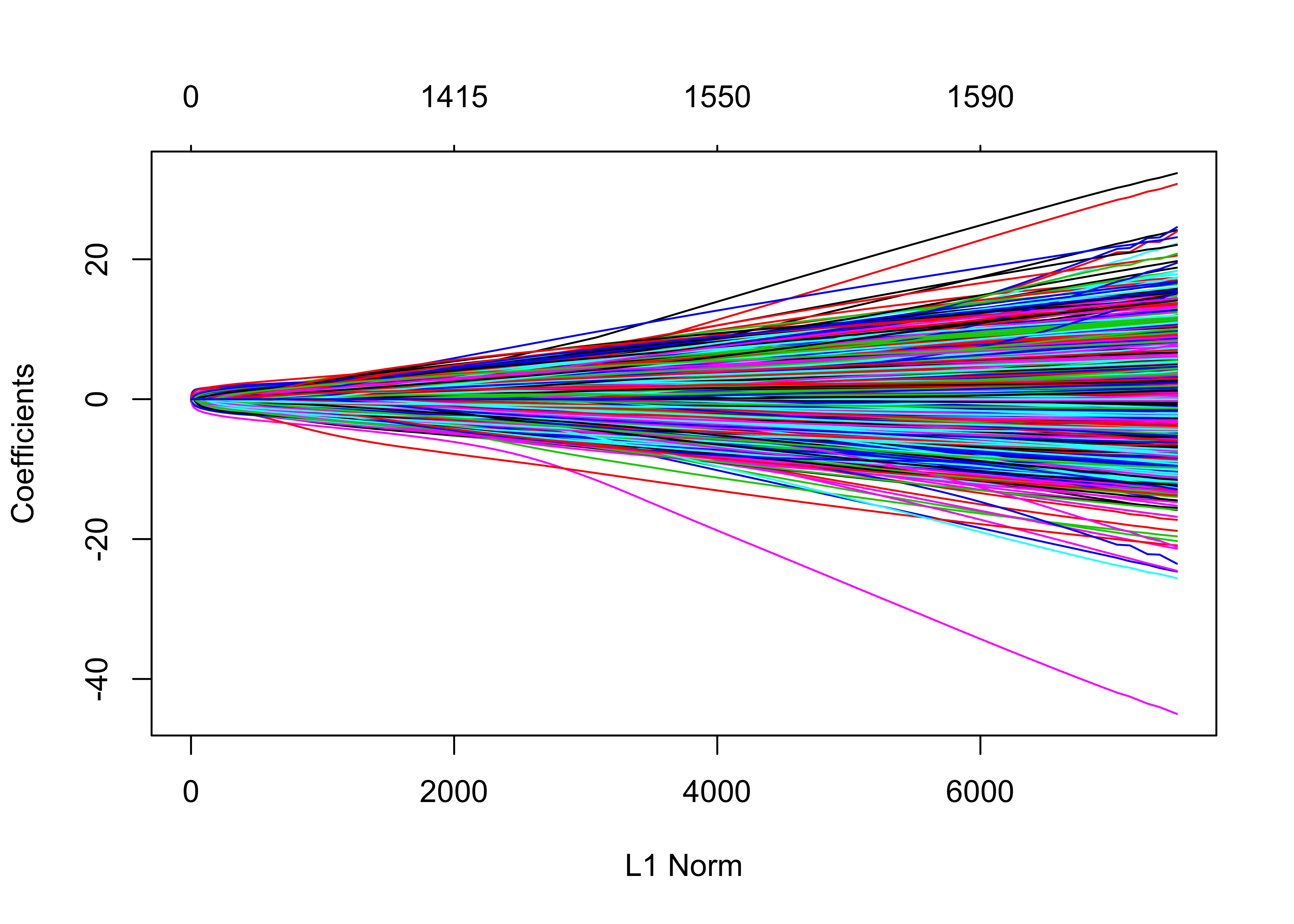

Understanding and evaluating our model

Those default plots are helpful, but we want to dig more deeply into our model and understand it better. For starters, what predictors are driving the model? Let’s use broom to check out the coefficients of the model, for the largest value of lambda with error within 1 standard error of the minimum.

library(broom)

coefs <- model$glmnet.fit %>%
  tidy() %>%
  filter(lambda == model$lambda.1se)

Which coefficents are the largest in size, in each direction?

coefs %>%
  group_by(estimate > 0) %>%
  top_n(10, abs(estimate)) %>%
  ungroup() %>%
  ggplot(aes(fct_reorder(term, estimate), estimate, fill = estimate > 0)) +
  geom_col(alpha = 0.8, show.legend = FALSE) +
  coord_flip() +
  labs(
    x = NULL,
    title = "Coefficients that increase/decrease probability the most",
    subtitle = "A document mentioning Martians is unlikely to be written by Jane Austen"
  )

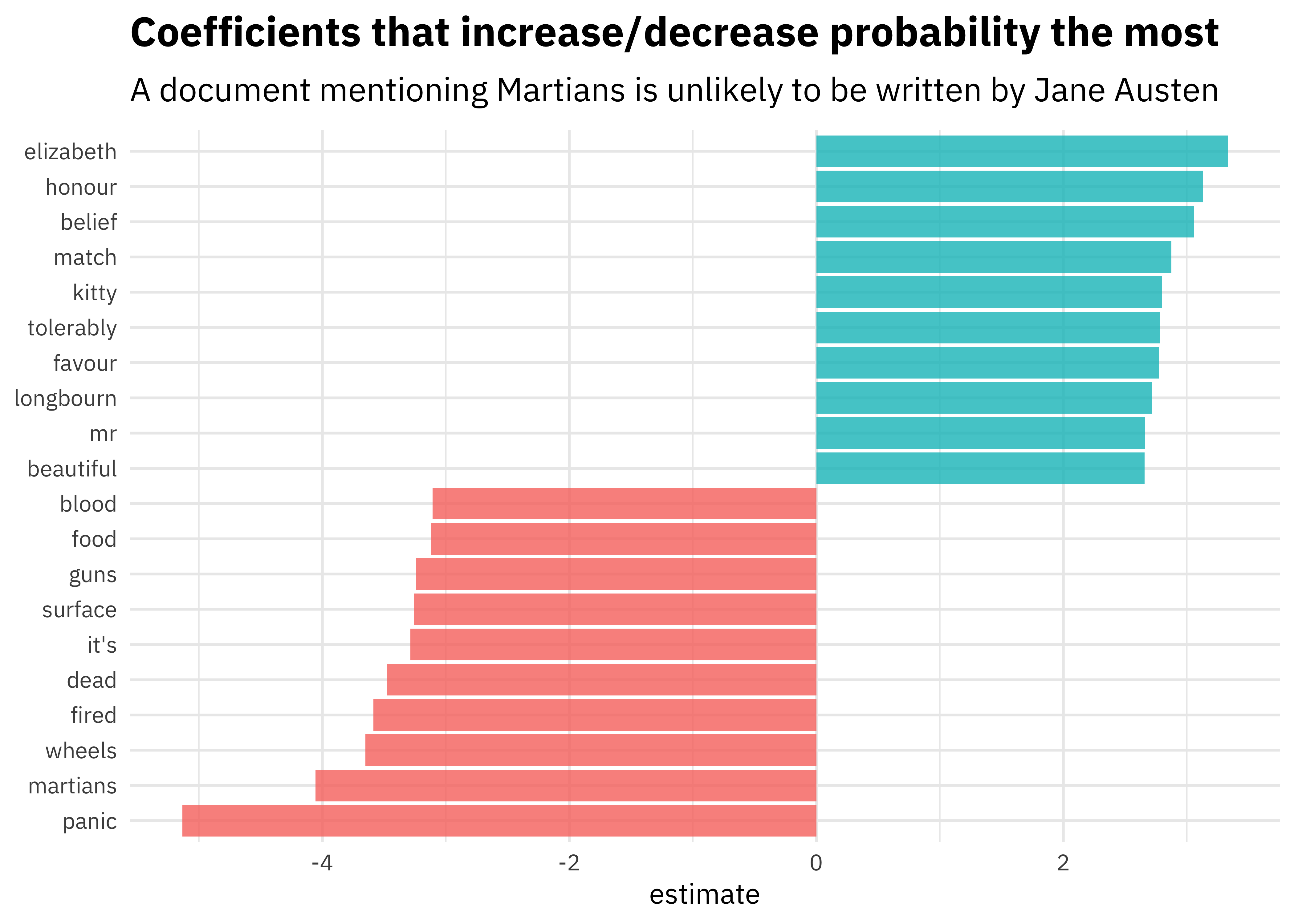
Makes sense, if you ask me!

We want to evaluate how well this model is doing using the test data that we held out and did not use for training the model. There are a couple steps to this, but we can deeply understand the performance using the model output and tidy data principles. Let’s create a dataframe that tells us, for each document in the test set, the probability of being written by Jane Austen.

intercept <- coefs %>%
  filter(term == "(Intercept)") %>%
  pull(estimate)

classifications <- tidy_books %>%
  inner_join(test_data) %>%
  inner_join(coefs, by = c("word" = "term")) %>%
  group_by(document) %>%
  summarize(score = sum(estimate)) %>%
  mutate(probability = plogis(intercept + score))

classifications

## # A tibble: 4,004 x 3
##    document  score probability
##       <int>  <dbl>       <dbl>
##  1        1 -1.83      0.170  
##  2        8 -1.02      0.317  
##  3       19  0.502     0.679  
##  4       21 -1.83      0.170  
##  5       25 -0.983     0.324  
##  6       28 -1.78      0.178  
##  7       30 -5.29      0.00643
##  8       31 -3.03      0.0584 
##  9       48  2.89      0.958  
## 10       49 -2.88      0.0675 
## # ... with 3,994 more rows

Now let’s use the yardstick package to calculate some model performance metrics. For example, what does the ROC curve look like?

library(yardstick)

comment_classes <- classifications %>%
  left_join(books %>%
    select(title, document), by = "document") %>%
  mutate(title = as.factor(title))

comment_classes %>%
  roc_curve(title, probability) %>%
  ggplot(aes(x = 1 - specificity, y = sensitivity)) +
  geom_line(
    color = "midnightblue",
    size = 1.5
  ) +
  geom_abline(
    lty = 2, alpha = 0.5,
    color = "gray50",
    size = 1.2
  ) +
  labs(
    title = "ROC curve for text classification using regularized regression",
    subtitle = "Predicting whether text was written by Jane Austen or H.G. Wells"
  )

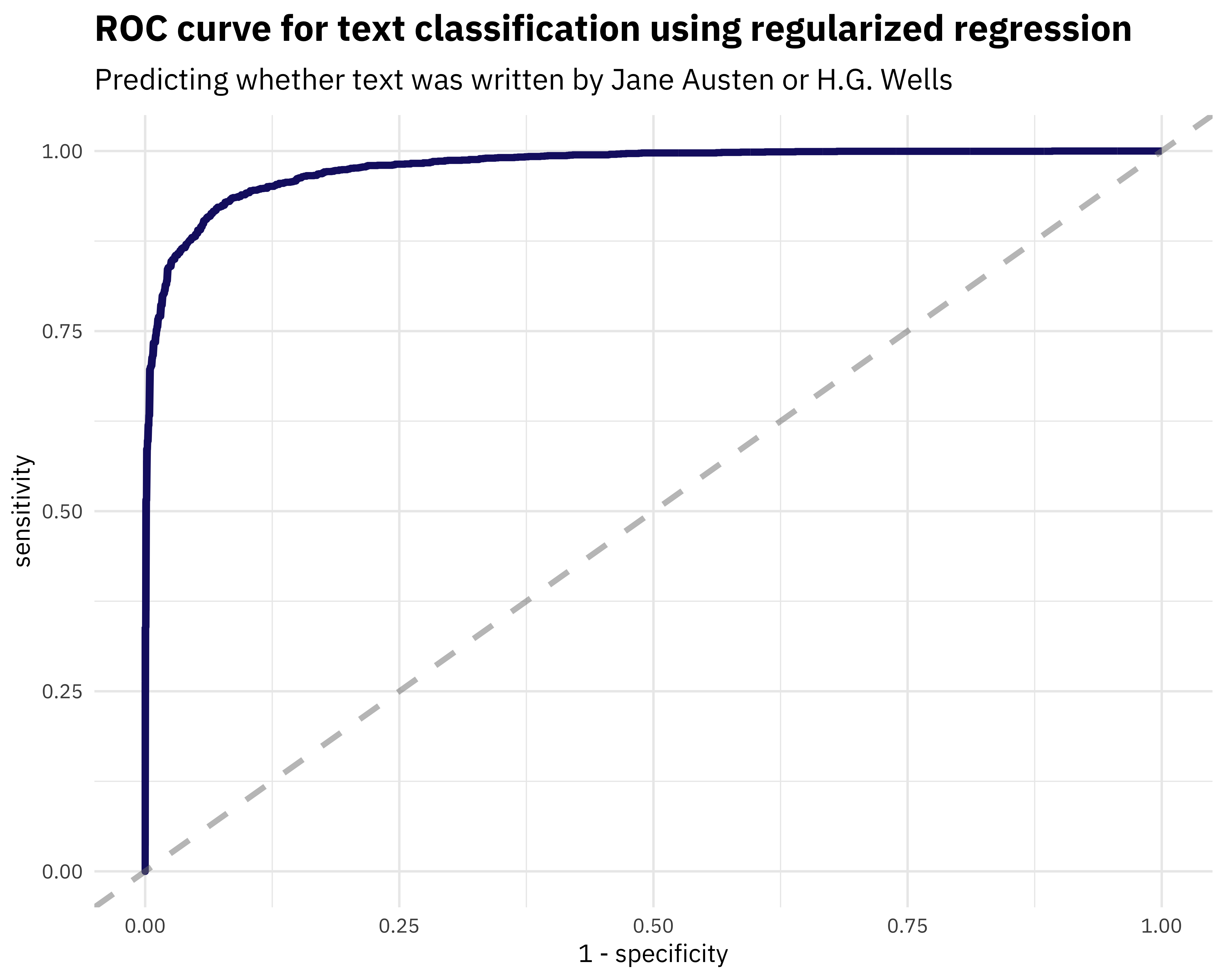
Looks pretty nice. What is the AUC on the test data?

comment_classes %>%
  roc_auc(title, probability)

## # A tibble: 1 x 3
##   .metric .estimator .estimate
##   <chr>   <chr>          <dbl>
## 1 roc_auc binary         0.978

Not shabby.

What about a confusion matrix? Let’s use probability of 0.5 as our cutoff point, for example.

comment_classes %>%
  mutate(
    prediction = case_when(
      probability > 0.5 ~ "Pride and Prejudice",
      TRUE ~ "The War of the Worlds"
    ),
    prediction = as.factor(prediction)
  ) %>%
  conf_mat(title, prediction)

##                        Truth
## Prediction              Pride and Prejudice The War of the Worlds
##   Pride and Prejudice                  2508                   180
##   The War of the Worlds                 122                  1194

More text from “The War of the Worlds” was misclassified with this particular cutoff point.

Let’s talk about these misclassifications. In the real world, it’s usually worth my while to understand a bit about both false negatives and false positives for my models. Which documents here were incorrectly predicted to be written by Jane Austen, at the extreme probability end?

comment_classes %>%
  filter(
    probability > .8,
    title == "The War of the Worlds"
  ) %>%
  sample_n(10) %>%
  inner_join(books %>%
    select(document, text)) %>%
  select(probability, text)

## # A tibble: 10 x 2
##    probability text                                                        
##          <dbl> <chr>                                                       
##  1       0.870 excited by the opening of the line of communication, which …
##  2       0.865 it was to attempt this crossing.  He turned to Miss Elphins…
##  3       0.892 the innkeeper, she would, I think, have urged me to stay in 
##  4       0.817 "\"No doubt lots who had money have gone away to France,\" …
##  5       0.877 The thought of the confined creature was so dreadful to him…
##  6       0.915 they did not wish to destroy the country but only to crush …
##  7       0.905 gunners, unseasoned artillery volunteers who ought never to…
##  8       0.851 verily believe that to the very end this spoiled child of l…
##  9       0.840 brim of which quivered and panted, and dropped saliva.  The…
## 10       0.829 was as if something turned over, and the point of view alte…

Some of these are quite short, and some of these I would have difficulty classifying as a human reader quite familiar with these texts.

Which documents here were incorrectly predicted to not be written by Jane Austen?

comment_classes %>%
  filter(
    probability < .3,
    title == "Pride and Prejudice"
  ) %>%
  sample_n(10) %>%
  inner_join(books %>%
    select(document, text)) %>%
  select(probability, text)

## # A tibble: 10 x 2
##    probability text                                                        
##          <dbl> <chr>                                                       
##  1      0.186  But here, by carrying with me one ceaseless source of regre…
##  2      0.124  arrival at Lambton, these visitors came. They had been walk…
##  3      0.178  of fancy, the streets of that gay bathing-place covered wit…
##  4      0.275  mention an officer above once a day, unless, by some cruel …
##  5      0.160  the slightest suspicion. I told him, moreover, that I belie…
##  6      0.212  behalf of the interested people who have probably been conc…
##  7      0.0639 occasional appearance of some trout in the water, and talki…
##  8      0.162  are instituted by the Church of England. As a clergyman, mo…
##  9      0.116  walking slowly towards the house.                           
## 10      0.210  it seems but a fortnight I declare; and yet there have been…

These are the texts that are from Pride and Prejudice but the model did not correctly identify as such.

The End

This workflow demonstrates how tidy data principles can be used not just for data cleaning and munging, but for sophisticated machine learning as well. I used my own tidytext package, and also a couple of packages from the tidymodels metapackage which provides lots of valuable functions and infrastructure for this kind of work. One thing I want to note is that my data was not in a tidy data structure the whole time during this process, and that is what I usually find myself doing in real world situations. I use tidy tools to clean and prepare data, then transform to a data structure like a sparse matrix for modeling, then tidy() the output of the machine learning algorithm so I can visualize it and understand it in other ways as well. We talk about this workflow in our book, and it’s one that serves me well in the real world. Thanks to Alex Hayes for feedback on an early version of this post. Let me know if you have any questions!